Driving through two-phase flow, Coriolis research, Advanced Instrumentation Research Group

Why does two-phase flow make flowtube control difficult? The main effect is a dramatic rise in the flowtube damping, perhaps by two orders of magnitude. Mechanical energy is lost in the interactions between compressible bubbles, fluid and flowtube walls, and the drive energy required to maintain oscillation rises sharply. Not only does the damping rise, but it varies rapidly, due to the chaotic nature of the interactions. Similarly, the frequency and amplitude of oscillation exhibit much greater variation than for single phase. The consequences for drive output are as follows:

•  Drive energy saturation. For any intrinsically safe flowtube, there is an absolute limit on the energy supplied to the driver(s) – for example 100mA. The default amplitude of oscillation may not be sustainable. While many in industry appreciate this limitation, it is widely and wrongly assumed that this is the main reason why flowtubes stall (For a counter- example, see below).       
  
  
• Drive gain saturation. Some positive feedback drives cannot exceed a maximum drive gain limit e.g. due to amplifier saturation. This means there is a maximum multiplier between the sensor amplitude in and the drive signal out. Suppose this limit is reached, and the flowtube damping rises again due to yet more gas in the two-phase flow mix. A further rise in drive current to compensate for the increased damping is not possible, due to drive saturation. As a consequence, the sensor amplitude starts to reduce, but this in turn leads, again because of drive saturation, to a drop in the drive signal output; the end result is a catastrophic collapse in oscillation amplitude.
  
  
• Poor tracking. The rapid changes in damping, amplitude, frequency and phase on the sensor signal require fast and accurate tracking by the transmitter in order to generate an appropriate drive signal. If the drive control update rate is simply too slow, the flowtube may stall due to inattention.

The UTC Transmitter

The Invensys UTC has developed new Coriolis meter transmitter technology to provide improved measurement performance and robustness. Several features provide improved flowtube control in the face of two-phase flow, including:

• Measurement and control updates every half drive cycle (typically every 6ms)
• Rapid dynamic response
• Synthesis of a pure sine wave with the required amplitude, frequency and phase characteristics, providing a highly adaptable and precise drive signal.
• A non-linear amplitude control algorithm providing stable oscillation [1].
• Selection of a sustainable set-point for the amplitude of oscillation during two-phase flow.
• The ability to generate counter-phase signals or so-called negative gain (see below)

Figure 1 demonstrates the precision of the flowtube control system via a sequence of set point changes over 3 orders of magnitude. The default amplitude is 0.3V. This is reduced to 30mV, 3mV, and finally 0.3mV, before these steps are reversed, all within 45s. Note that 0.3V corresponds to a physical oscillation of 0.6 mm. The graph also shows the drive current requirements during these steps, which reduces linearly with amplitude.

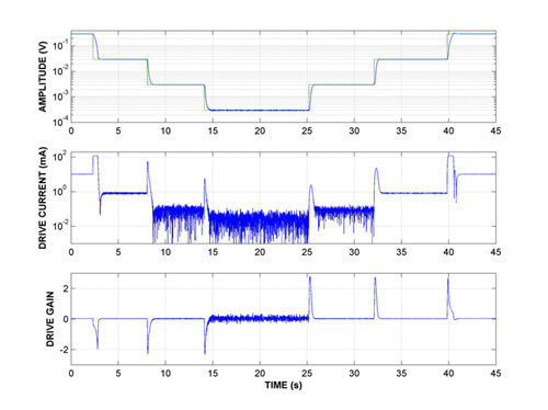
Figure 1. Digital drive control of flowtube as amplitude of oscillation is reduced by three orders of magnitude.

The drive gain is defined as the ratio of the drive current to the amplitude of oscillation. Its mean value is approximately constant when the amplitude is steady. During set-point changes it exhibits large swings. Negative gain values are generated by the control algorithm when it is desirable to reduce the amplitude of oscillation rapidly. The transmitter does this by generating drive signals that are 180 degrees out of phase with the sensor signals, thus opposing drive motion. This is useful not only for effecting set-point changes, but also for maintaining flowtube stability at low amplitudes (e.g. t=15-25s) and with high damping (e.g. two-phase flow).

Figure 2 shows in more detail the sensor voltage and drive output when the amplitude of oscillation is 0.3mV. Several features of the drive synthesis algorithm are demonstrated. The drive and sensor signals are substantially in phase with each other. The amplitude of the drive signal is updated every half cycle. Occasionally a negative gain value is used, in which case consecutive half-cycles of the drive output have the same polarity. These techniques are effective: the sensor amplitude stays within 1% of the set-point, despite operating at only 0.1% of the normal amplitude of oscillation.

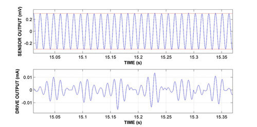
Figure 2. Detail of drive signal to maintain flowbue oscillation at 0.1% of conventional setpoint.

Figure 3 illustrates how these features are used to maintain flowtube oscillation during two-phase flow, and when the flowtube is drained and refilled. This is achieved despite an artificially low maximum drive current of only 20mA – a more typical intrinsically safe limit would be 80mA. Initially (t=0s) the process fluid is single phase, and the amplitude of oscillation is the default value of 0.3V, maintained using 9mA per drive. Between t=3s and t=30s, there is a surge of air in the process fluid, as indicated by the density which drops to approximately 700kg/m³. This causes a rapid rise in flowtube damping and hence the drive current needed to maintain flowtube oscillation. As the drive current limit of 20mA is reached, a new amplitude set-point is selected, and again at 17s, as indicated by the dashed line on the sensor amplitude graph. After t=35s, the process fluid becomes single phase and the drive gain returns to its conventional value. It is thus possible to revert to the default set-point of 0.3V. This is achieved (t=35-38s) using maximum drive current; with a less severe current limit the amplitude rise would occur more rapidly. At t=50s, a new disturbance occurs: the pump is switched off, causing process fluid to drain from the meter. Accordingly the density drops rapidly. The draining process introduces a high degree of damping for several seconds, and so at first a reduced set-point is adopted; however by t=55s draining is completed, and the default set-point is restored. However, at this point the pump is switched on again and the flow meter experiences the hydraulic shock caused by the onset of flow. By t=65s equilibrium has been restored, damping has reduced and the default amplitude of 0.3V has been reinstated. Note that the flowmeter maintains operation and continues to generate measurement data throughout these transients. Note also that this was achieved with only 20mA of drive current: with a more realistic limit of 80mA much tighter amplitude control is achieved.

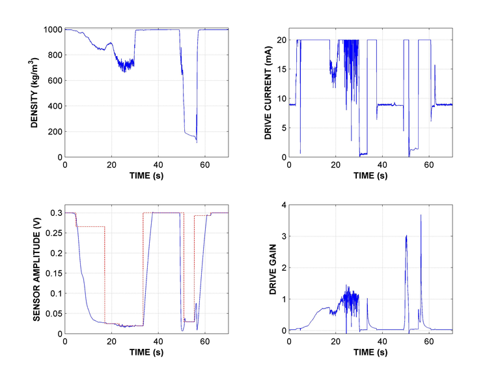
Figure 3: Flowtube amplitude control through two-phase flow

References

[1] Clarke, DW, “Non-linear control of the oscillation amplitude of a Coriolis mass-flow meter”, European Journal of Control, Vol. 4, No. 3, pp196-207, 1998.