Dynamic Response, Coriolis research, Advanced Instrumentation Research Group

 

In their ISA 2002 paper [1], Wiklund and Peluso explain the growing importance of the dynamic response of a flowmeter, which indicates how rapidly it is able to track changes in flowrate. The authors modelled the dynamic response of several flowmeter technologies (differential pressure (DP) with orifice plate, electromagnetic, vortex and Coriolis), testing the products of several manufacturers. Figure 1 shows, for the fastest meter in each class, the response to an instantaneous unit step change in the true flowrate, based on the parameter values reported in [1]. As Fig 1 shows, there are two aspects to the dynamic response – an initial ‘deadtime’, where there is no change in output, and then a first or second-order response towards the new steady-state value. In [1], DP and orifice plate is shown to have the fastest response, while Coriolis has the slowest. However, the fastest response curve in Fig 1, superimposed on the data from [1] is the performance of a prototype Coriolis meter developed by the Oxford UTC. The dead time is 10-16ms, and the new steady state value is achieved within a further 20-30ms.

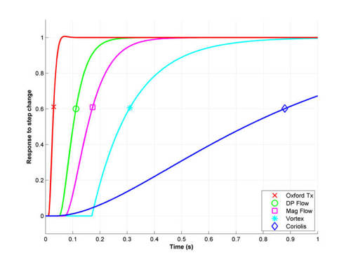
Figure 1. Dynamic response of flow meters to a unit step change in flowrate (derived from [1]).

Figure 2 shows experimental data collected at Brunel University showing the response of the Oxford transmitter, working with a 25mm bent flowtube. The water flow test rig at Brunel [2] can generate fast steps in flow e.g. from 0.6kg/s to 0.1 kg/s within 3ms. An electromagnetic flowmeter with continuous dc excitation gives a dynamically responsive indication of the time-course of the step. Note however, that this is at the expense of DC accuracy – the fast response electromagnetic flowmeter is not viable as an industrial instrument, only as a laboratory tool. The Coriolis pulse output and the electromagnetic flowmeter are recorded simultaneously. In fig. 2, the observed pulse output is shown after a fast step change in massflow. The pulse output has a staircase form as updates are provided twice per drive cycle, i.e. every 6ms. The electromagnetic flowmeter provides the reference time-history for the massflow step, which takes place at t = 0ms. The transmitter output responds at t = 12ms and the step is completed some 23ms later.

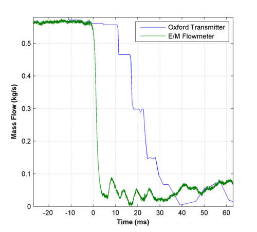
Figure 2. Experimental Dynamic response of Oxford Coriolis transmitter carried out at Brunel University.

 

Sources of Delay

 

A Coriolis meter is partitioned into two sections: the flowtube and the transmitter. The flowtube is a mechanical component providing the pipework through which the process fluid flows, including the measurement section which is able to vibrate, along with (usually coil-based) sensors and driver(s) to monitor and maintain the flowtube vibration. The transmitter is essentially an electronic device with electrical connections to the sensors and drivers of the flowtube. The tasks of the transmitter are to initiate and maintain flowtube vibration and to extract mass flow, density and possibly other process data from the sensor signals.

Here the term ‘delay’ will be used to denote both dead-time and step response elements of the dynamic response of the meter.

Research at Brunel [3] has established that the mechanical response of the flowtube to a step change in flow rate cannot be observed over a period of less than one complete cycle of the driven motion. Thus, roughly speaking, a flowtube oscillating at 100Hz cannot respond more rapidly than 10ms, while a 1kHz flowtube might respond in a millisecond. As Fig. 1 illustrates, however, the actual response of commercial flowmeters is much slower: the major sources of delay lie in the transmitter.

Flowtube design has other consequences. The design constraints for a straight (as opposed to a bent) geometry lead to high frequency, low amplitude oscillations, providing mixed benefits from a dynamic response perspective. While a high frequency (say 800Hz vs. 80Hz) is desirable, the lower sensor signal amplitude (say 30mV vs. 300mV) and lower phase difference range (say 0.4 degrees vs. 4.0 degrees) may result in a lower signal-to-noise ratio. As discussed below, this may necessitate measurement filtering, which is one of the most significant causes of transmitter-induced delay.

Within the Coriolis transmitter, data processing occurs in several stages. The sensor signals from the flowtube are usually sampled via analog-to-digital (ADC) converters in the transmitter. In some cases additional filtering is applied. Each step introduces some delay. Within the transmitter processor, measurement calculations are not carried out continuously, but typically every one or more drive cycles. Clearly any step change in flow will on average be delayed by half the measurement update period.

In many industrial applications, the most important yardstick of dynamic response is the time taken for a change in flow to be communicated via the transmitter outputs (e.g. 4-20mA, pulse or fieldbus). Again, an update to the transmitter output circuitry is not necessarily provided every time a new measurement value is calculated. Given the conventional scanning rates of industrial control systems, it is more typical for updates to be provided at a rate of 10Hz or slower. The most accurate representation of the measurement data over the last (say) 100ms would be its average over the measurement update period. This introduces on average (say) 50ms delay in the response of the flowmeter. Furthermore, it is common to introduce additional filtering at this stage, in order to smooth the reported measurement value. With time constants of typically 40-1000 ms, such filtering can be the most significant influence in the dynamic response of commercial meters.

• With 4-20mA communications, the flow rate is mapped onto an analog current signal between 4 and 20mA.There is no delay in propagating the signal to the monitoring system, but there can be delay in the analog current circuitry.
• Pulse (frequency) output consists of a square wave signal in which the frequency of the pulse stream indicates the flowrate. This has some of the advantages of 4-20mA, being simple, unidirectional and continuous, while the discrete signal edges give some benefits of digital transmission, including higher precision. There are delays inherent in this technique, however. Typically the upper limit on the output is about 10kHz.  Also zero flow is often mapped onto zero Hz, so that at low flowrates there can be significant propagation delays due to the timing between edges – for example at 200Hz there is a 5ms period between rising edges. If the pulse output frequency is only updated after each rising edge (say), then this can lead to several milliseconds delay in propagating a step change from a low to a high flow value.      
• Various digital communication protocols (e.g. Profibus, FF, HART) allow the transmission of measurement data in floating point format, with no loss of precision. Again, typically in the process industries, measurement data is transmitted no more frequently than every 100ms, which places a lower limit on the overall dynamic response of the meters

There is little doubt that the adoption of standardised, high-speed (e.g. supporting 1000 updates/s) digital communications will benefit applications where dynamic response is important. However, until such standards emerge, for applications where dynamic response is paramount, there is much to be said for the speed offered by a precise pulse/frequency output coupled to a fast PLC (with a cycle time of say 1ms). The Oxford Group has developed a pulse output algorithm [4,5] which over 1 second is precise to 1 part in 10 million at any frequency. Results cited in this paper have been generated using this pulse output.

 

Delay in the Oxford UTC Transmitter

 

The UTC and its predecessor, the Sensor Validation Research Group at the University of Oxford has developed the concept of the Self-Validating (SEVA) sensor for the last 20 years. Analysis of the fault modes of earlier Coriolis transmitters has led to an all-digital design which eliminates certain classes of fault (e.g. stalling with two-phase flow) and which offers a much improved dynamic response. The transmitter is ‘digital’ in that all components, other than elementary front end circuitry, are digital devices. This facilitates high speed, high precision measurement and control calculations. When driving a B-shaped Coriolis flowtube, measurement and control updates are provided every half-cycle (i.e. at 150-200Hz). However, the transmitter can drive other flowtube designs, including straight tube geometries, with drive frequencies of up to 1kHz. It has a 32 bit processor with hardware floating point, and uses a Field Programmable Gate Array (FPGA) – a programmable logic chip - for real-time aspects of flowtube control, for example drive waveform synthesis. A third useful digital technology is the audio codec (combined stereo ADC and DAC – two sensor channels in and two drive channels out) providing 24bit data at 40kHz.

An estimate of the dead time of the prototype transmitter is as follows. Although the codec samples at 40kHz, there is a 61 sample ‘group delay’ between input and output, equivalent to 1.5ms dead time. Low-pass filtering in the FPGA introduces an additional 1ms delay. For a typical drive frequency of 80Hz, there is a delay of approximately 6ms (per half-cycle) for data accumulation. The processor required a further 1.5ms to perform the measurement calculation. The pulse output is updated immediately after each measurement calculation has been completed, and there are negligible delays (<1ms) in propagating a step change in flowrate through to the pulse output, even for low flowrates. As discussed below, the high precision of the measurement calculation and frequency generation means that no averaging or filtering is required to provide a smooth measurement output, which results in a much improved dynamic response. Overall, this analysis suggests a total dead time of 10-16ms from sensor signal input through to pulse output, depending on where in the half-cycle a step change occurs. This estimate is similar to the theoretical limit suggested by Brunel for an 80Hz drive frequency, and is confirmed by experimental results (Fig 2).

These techniques have been extended to higher frequency Coriolis flowtubes with straight geometries, demonstrating a dynamic response of 3.8ms [6].

 

Example: Filling System

 

A UK manufacturer of filling machines has using digital coriolis metering in batch filling products. This has proved successful with double diaphragm pumps in industrial applications. Fig. 3 shows a small filling system consisting of a 15mm flowtube and transmitter, gravity-fed flow, and a fast PLC controlling the shutoff valve.

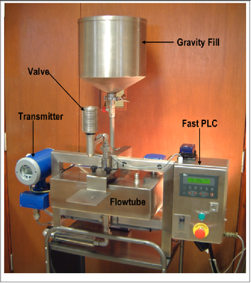
Figure 3. Filling system used for short batch trials.

The pulse output of the transmitter is monitored every millisecond by the PLC. When the target total flow is achieved, the valve is shut. The target total flow includes the so-called “in-flight” adjustment which accounts for additional flow attributable to flowtube and valve shutoff delay.

Figure 4 shows the time profiles of short batches carried out on the rig, ranging in size from 1g to 6g. Inside the Coriolis meter transmitter, measurement updates occur every 6ms, as indicated by the symbols on each line. Superimposing the time series of separate runs on the same time axis allows comparisons of the flow profiles.

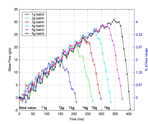
Figure 4. Time profiles of 1g - 6g fast batches

For example, the 1g fill takes approximately 200ms; the PLC sends the shut valve command after only 80ms, after which a further 120ms are required for the valve to compete shutoff. The maximum flow is 15g/s, or 2% of the flow range of the meter. The 6g fill takes 400ms; the PLC sends the shut valve command after 315ms, which requires a further 85ms to complete. The maximum flow is 30g/s, or 4% of the flow range of the meter.

The repeatability of this system is demonstrated in the following table, which shows the weighscale total for 25 consecutive 6g runs.

Consecutive 6g, 400ms batch totals (g)
5.99	5.97	5.98	5.99	5.95
5.97	5.98	6.01	5.99	5.96
6.02	5.99	6.00	6.01	5.99
5.97	5.98	6.01	5.96	5.98
6.00	6.02	6.01	6.02	5.96
Min = 5.95, Max = 6.02, Repeatability = 0.07g

The repeatability over 25 consecutive 1g, 200ms trials was 0.08g. Clearly, this performance is attributable in part to the short dead time and good dynamic response of the meter.

 

References

[1] Wiklund D. Peluso M.: Quantifying and specifying the dynamic response of flowmeters, ISA 2002 Technical Conference.

[2]  Henry, M.P., Clark, C., Duta, M., Cheesewright, R., Tombs, M.: Response of a Coriolis mass flow meter to step changes in flow rate, Flow Measurement and Instrumentation, Vol. 14 , pp 109-118, 2003.

[3] Cheesewright R, Clark C, Belhadj A., Hou Y Y.: The dynamic response of Coriolis mass flow meters, Journal of Fluids and Structures, 18, pp165-178, 2003.

[4] Henry, MP: “Frequency output generation through alternating between selected frequencies”, US Patent No. 6,914,463, July 2005.

[5]  Zamora, ME, Wu, H, and Henry, MP. “An FPGA Implementation of Frequency Output”, IEEE Transactions on Industrial Electronics , Vol 56, No. 3, March  2009.

[6] Clark C, Zamora, M, Cheesewright, R, Henry M., The dynamic performance of a new ultra-fast response Coriolis flow meter, Flow Measurement and Instrumentation 17 (2006), pp391-98, doi:10.1016/j.flowmeasinst.2006.07.002