Bandpass Filtering for Prism Technology, Advanced Instrumentation Research Group

The following example illustrates how bandpass filters can be constructed using pairs of Prisms in series.

The figure below shows the variation in gain against frequency for the Prism output G_s^h  with h = 1, .., 12.

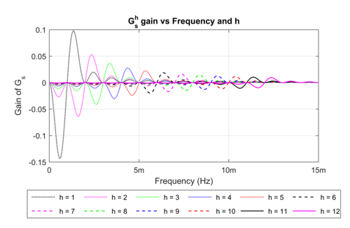
For each h there is a positive and a negative peak, with the negative peak occurring in the range [h-1, h] x m Hz while the positive peak appears in the range [h, h+1] x m Hz.

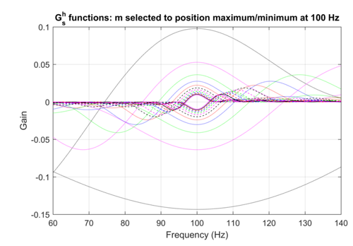
The next figure below shows how, by selecting the appropriate value of m in each case, a family of G_s^h functions can be created with either a positive or negative peak at some arbitrary frequency, here 100 Hz. For each value of h a pair of G_s^h functions is created: one with its positive peak positioned at 100 Hz and the other with its negative peak at 100 Hz.

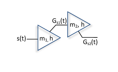
By placing two Prisms in series, with suitably selected values of m and a common h value, as illustrated below, simple bandpass filters can be created.

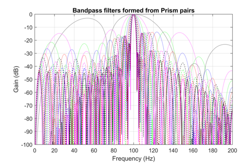
The next figure below shows the filtering performance of such Prism pairs. A sequence of bandpass filters are produced with, for increasing h, a narrowing passband around the chosen central frequency.

Further pairs of Prisms may be networked in series to increase the attenuation of frequencies outside the desired passband. For example the figure below shows a bandpass filter consisting of 3 pairs of Prisms in series.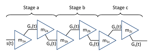

Typically, such filtering would be followed by a Prism-based tracker to obtain frequency, phase and/or amplitude information from the reduced-bandwidth signal.

Using three pairs of Prisms, powerful bandpass filters can be constructed, whereby both the design and computational costs are low. An example of the theoretical and numerical performance of such a filter is shown below.

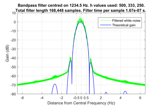
Here the sampling rate fs is 48 kHz, and an arbitrary central frequency of 1234.5 Hz has been selected. Pairs of Prisms with h values of 500, 333 and 250 have been networked in series to create a filter with a passband (to -10 dB) of ± 0.5 Hz. The total filter length is 168,448 samples, but the computational burden is low, as only six Prism evaluations are needed for each sample, and only the G_s^h output is calculated for each Prism. The figure above also shows that, when applied numerically to white noise, the filter delivers its theoretical performance. The computational requirement is 1.67e-7s per sample, so that the real-time 48 kHz throughout requires only 0.8% of an i7 core. Perhaps more importantly, the design and instantiation of such a bandpass filter is straightforward, so that any moderately powerful device could create one or more such filters, adjusting the central frequency and/or the pass bandwidth upon request or with changing environmental conditions.